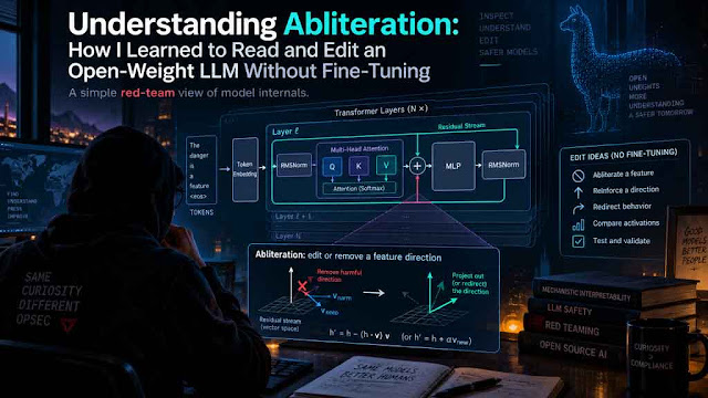
Updated on October 3, 2026

A practical red-teamer's guide to layers, Q/K/V/O, hidden states, behavior directions, steering, ablation, weight orthogonalization, and what I learned experimenting with Qwen

When I first started looking into LLM abliteration, I had a fairly simple question:

If I have the weights of an open model, where exactly is a behavior such as refusal, verbosity, or conciseness stored, and how do I change it?

At first I imagined there might be something like a "refusal matrix."

Find the matrix. Change some numbers. Save the model.

It turns out that this mental model is much too simple.

An LLM contains billions of parameters, but behavior does not usually map cleanly to one parameter, one matrix, or even one transformer layer. What we can often find instead is a direction in the model's activation space that correlates with a behavior.

Once we find such a direction, we can experimentally push the model along it, remove it, watch whether later layers recreate it, and eventually, when the evidence supports it, modify the matrices that write into that space.

That family of techniques is what people usually mean when they talk about abliteration.

The technique became widely known following research showing that refusal behavior in a number of chat models could be associated with a surprisingly low-dimensional, in many cases effectively one-dimensional, direction in the residual stream. Removing that direction reduced refusal, while adding it could induce refusal even for harmless requests. arXiv

The community later popularized the term abliteration for using this observation to identify a direction and project it out of activations or weights. Hugging Face

As a red teamer, I found the idea fascinating because it is very different from fine-tuning.

There is no optimizer.

There is no backpropagation.

There is no new training dataset in the normal fine-tuning sense.

We are doing something closer to reverse engineering.

My workflow became:

observe behavior
      ↓
capture internal state
      ↓
find what differs
      ↓
test whether the difference is causal
      ↓
find where it matters
      ↓
remove it temporarily
      ↓
check whether the network rebuilds it
      ↓
only then consider modifying weights

That distinction is important because finding a behavior in an activation does not prove that activation causes the behavior.

That lesson ended up being one of the most interesting findings from my Qwen experiments.

---

What I mean by "uncensored"

One motivation for my research is building a local model for authorized security and red-team work that does not reflexively refuse legitimate security research tasks.

I use the word uncensored carefully.

I do not mean that every safety mechanism in an LLM can be reduced to one switch. I also do not assume that there is one universal "refusal matrix."

What I am trying to understand is much more specific:

Can refusal-associated behavior be experimentally located, measured, causally manipulated, and selectively reduced without retraining the entire model?

That is especially useful for security research because model alignment can sometimes interfere with legitimate adversarial testing, exploit analysis, malware classification, payload analysis, offensive-security simulation, and other work where the content itself looks suspicious even when the context is authorized.

The same methodology also lets me study completely benign behaviors.

In fact, I deliberately began with verbosity versus conciseness rather than refusal.

Why?

Because if I cannot reliably discover something as easy to observe as:

verbose answer
versus
compact answer

then I certainly should not trust myself to locate something more complicated like refusal.

That verbosity experiment turned out to teach me much more about transformer internals than I expected.

---

Before abliteration: understand what is actually inside the model

The model I used for the experiment was:

Qwen/Qwen2.5-1.5B-Instruct

When I inspected its configuration, I got:

Hidden size:       1536
Layers:            28
Intermediate size: 8960
Attention heads:   12
KV heads:          2
Vocabulary:        151936

Those are the actual values from the model I tested. Pasted text

Before going any further, we need to understand what each of those numbers means.

---

The most important number: 1536

I kept seeing:

1536

everywhere.

For example:

q_proj        [1536, 1536]
o_proj        [1536, 1536]

gate_proj     [8960, 1536]
up_proj       [8960, 1536]
down_proj     [1536, 8960]

At first this looks like a random implementation detail.

It is not.

1536 is the model's hidden size, often called:

d_model

The simplest way to understand it is:

At any point in the main transformer stream, each token is represented by 1536 numbers.

Imagine the token:

"security"

Internally, the model is not carrying the word "security" around.

It is carrying something more like:

[
   0.14,
  -0.82,
   1.31,
   ...
   0.09
]

except there are 1536 values.

So:

one token
    ↓
1536-dimensional vector

The entire transformer keeps transforming that vector.

---

The embedding matrix

The Qwen checkpoint contained:

model.embed_tokens.weight
[151936, 1536]

Pasted text

This makes sense once we know the vocabulary size.

There are:

151,936 possible tokens

and each token receives a:

1536-dimensional embedding

So conceptually:

token ID
   ↓
lookup table
   ↓
1536 floating-point values

The embedding matrix is therefore:

[vocabulary_size, hidden_size]

[151936, 1536]

---

What is a transformer layer?

Qwen2.5-1.5B has:

28 transformer layers

Think of the model roughly like this:

tokens
  ↓
embedding
  ↓
Layer 0
  ↓
Layer 1
  ↓
Layer 2
  ↓
...
  ↓
Layer 27
  ↓
final normalization
  ↓
vocabulary probabilities

Each layer receives a hidden state with width 1536.

Each layer modifies it.

The width remains:

1536

because every layer must hand a compatible representation to the next layer.

The meaning encoded in those 1536 values changes dramatically as the token travels through the network.

Early layers might encode basic lexical or syntactic information.

Middle layers may contain richer concepts and task-related features.

Later layers increasingly transform those representations toward the next-token prediction.

Do not interpret this as a rigid layer-by-layer job description. Transformers are highly distributed systems.

---

The residual stream

The concept that made LLM abliteration click for me was the residual stream.

Instead of imagining every transformer layer as destroying its input and creating something completely new, imagine a shared information highway:

        Residual Stream
              │
              ▼
       ┌─────────────┐
       │  Attention  │
       └──────┬──────┘
              │
              +
              │
       Residual Stream
              │
              ▼
       ┌─────────────┐
       │     MLP     │
       └──────┬──────┘
              │
              +
              │
       Residual Stream

Attention writes information into it.

The MLP writes information into it.

Then the next transformer block receives it.

For Qwen, that residual stream has width:

1536

This is extremely important because the behavior direction we discovered also has width:

1536

So we can mathematically ask:

How much of the current residual state points in the "verbose" direction?

That is the core idea behind much of the experiment.

---

What are Q, K, V and O?

Inside the attention system we have:

q_proj
k_proj
v_proj
o_proj

These stand for:

Name	Meaning	Simple interpretation
Q	Query	What am I looking for?
K	Key	What information do I contain?
V	Value	What information should I contribute?
O	Output	Write the attention result back into the residual stream

For this Qwen model the actual shapes are:

q_proj.weight    [1536, 1536]

k_proj.weight    [256, 1536]

v_proj.weight    [256, 1536]

o_proj.weight    [1536, 1536]

Pasted text

PyTorch stores a Linear layer's weight as:

[out_features, in_features]

So:

q_proj [1536,1536]

means:

1536 values come in
1536 query values come out

while:

k_proj [256,1536]

means:

1536 values come in
256 key values come out

---

Why are K and V only 256?

Qwen has:

12 attention heads
2 KV heads

and each head is:

128 dimensions

because:

1536 / 12 = 128

Therefore the query projection needs:

12 × 128 = 1536

values.

But keys and values have only two heads:

2 × 128 = 256

That is why:

k_proj = [256,1536]
v_proj = [256,1536]

This is called Grouped Query Attention, or GQA.

Twelve query heads share two sets of key/value heads.

In simplified terms:

Query heads

Q0 Q1 Q2 Q3 Q4 Q5 ─────► KV head 0
Q6 Q7 Q8 Q9 Q10 Q11 ───► KV head 1

This saves memory and makes inference faster.

---

What is an attention head?

An attention head is essentially one independent attention calculation.

Very roughly:

hidden state
     ↓
   Q K V
     ↓
Q compares with K
     ↓
attention scores
     ↓
scores weight V
     ↓
result

Mathematically:

$$Attention(Q,K,V) = softmax\left(\frac{QK^T}{\sqrt{d}}\right)V$$

The part:

$$QK^T$$

produces the attention scores.

That score answers something like:

How relevant is token B to what token A currently needs?

If I have:

The attacker obtained the password because ___ was weak

different tokens can attend to:

attacker
password
because
weak

with different strengths.

Attention heads let the model selectively combine information from previous tokens.

---

What does `o_proj` do?

After the attention heads finish their work, their result must go back into the main 1536 dimensional residual stream.

That is the job of:

o_proj

For Qwen:

o_proj.weight
[1536,1536]

You can think of it as:

attention's internal representation
          ↓
        o_proj
          ↓
1536-dimensional residual contribution

This makes o_proj interesting for abliteration.

It is a writer into the residual stream.

---

The MLP side: gate, up and down

The other major part of every transformer block is the MLP.

For Qwen:

gate_proj    [8960,1536]
up_proj      [8960,1536]

down_proj    [1536,8960]

Pasted text

Notice what happens:

1536
 ↓
8960
 ↓
1536

The MLP temporarily expands the representation into a much larger feature space.

A simplified Qwen-style gated MLP looks roughly like:

gate = silu(gate_proj(x))
up   = up_proj(x)

hidden = gate * up

output = down_proj(hidden)

So:

gate_proj

decides which intermediate features become active.

up_proj

creates those candidate features.

down_proj

compresses the resulting 8960 features back into the model's normal:

1536-dimensional residual space

That makes:

mlp.down_proj

another important residual writer.

---

Why we care about `o_proj` and `down_proj`

The two matrices:

self_attn.o_proj
mlp.down_proj

both produce outputs with width:

1536

and both write directly into the residual stream.

That does not automatically mean they control whatever behavior we are studying.

But if we discover a behavior direction:

d ∈ R^1536

these matrices are natural places to investigate.

This is very different from blindly modifying:

q_proj
k_proj
v_proj
gate_proj

just because they happen to be matrices.

We need a mechanistic reason for choosing the matrix.

---

A simple script to inspect an open model

This is the first script I would recommend running on any Hugging Face model to aid in understanding the model for LLM abliteration.

from transformers import AutoConfig, AutoModelForCausalLM

MODEL_ID = "Qwen/Qwen2.5-1.5B-Instruct"

config = AutoConfig.from_pretrained(MODEL_ID)

print("=== CONFIG ===")
print("Hidden size:", config.hidden_size)
print("Layers:", config.num_hidden_layers)
print("Intermediate size:", config.intermediate_size)
print("Attention heads:", config.num_attention_heads)

if hasattr(config, "num_key_value_heads"):
    print("KV heads:", config.num_key_value_heads)

print("Vocabulary:", config.vocab_size)


print("\nLoading model...")

model = AutoModelForCausalLM.from_pretrained(
    MODEL_ID,
    dtype="auto",
    device_map="cpu",
)


print("\n=== PARAMETERS ===")

for name, param in model.named_parameters():
    print(
        f"{name:70s}",
        str(list(param.shape)):20s,
        param.dtype,
    )

For Qwen this produced structures such as:

model.layers.16.self_attn.q_proj.weight
[1536,1536]

model.layers.16.self_attn.k_proj.weight
[256,1536]

model.layers.16.self_attn.v_proj.weight
[256,1536]

model.layers.16.self_attn.o_proj.weight
[1536,1536]

model.layers.16.mlp.gate_proj.weight
[8960,1536]

model.layers.16.mlp.up_proj.weight
[8960,1536]

model.layers.16.mlp.down_proj.weight
[1536,8960]

The checkpoint confirmed the same architecture throughout all 28 transformer blocks. Pasted text

---

How do I see the actual matrix values?

A matrix is not abstract. It contains actual learned floating-point values.

For example:

layer = model.model.layers[16]

W = (
    layer
    .self_attn
    .o_proj
    .weight
    .detach()
    .float()
    .cpu()
)

print(W.shape)

print("\nTop-left 5x5:")
print(W[:5, :5])

print("\nStatistics:")
print("mean:", W.mean().item())
print("std :", W.std().item())
print("norm:", W.norm().item())

You may see something like:

tensor([
    [ 0.0041, -0.0182, ...],
    [-0.0076,  0.0028, ...],
    ...
])

Those numbers came from training.

We are not going to manually guess new numbers.

Abliteration works because we calculate a geometric transformation based on measured activations, then apply that transformation to the matrix.

---

We do not find a "refusal matrix"

This distinction is important enough to state directly.

There usually is no parameter called:

refusal.weight

or:

verbosity_matrix

Instead we observe the model while it exhibits two different behaviors.

For my experiment:

verbose
versus
concise

For refusal-associated research it could be:

refusal-associated condition
versus
answering condition

Then we ask:

What consistently changes inside the model between these conditions?

---

This is another concept that initially confused me.

Weights are persistent:

q_proj.weight
down_proj.weight
...

They live in the checkpoint.

Activations exist while the model is running.

For one prompt you might get:

Layer 16 activation:
[1536 numbers]

For another prompt:

Layer 16 activation:
[different 1536 numbers]

So:

weights
  +
input
  ↓
activation

Abliteration normally starts by studying the activations.

Only much later might we update the weights.

---

Capturing a layer's activation

A PyTorch forward hook is a convenient way to see the output of a transformer block.

For example:

import torch

layer = model.model.layers[16]

captured = {}


def hook(module, inputs, output):

    hidden = (
        output[0]
        if isinstance(output, tuple)
        else output
    )

    captured["activation"] = (
        hidden[:, -1, :]
        .detach()
        .float()
        .cpu()
    )


handle = layer.register_forward_hook(hook)

Then run the model.

Afterward:

print(
    captured["activation"].shape
)

For a single prompt:

[1,1536]

The -1 means:

last token position

So we have captured a 1536-dimensional representation of the current prompt at Layer 16.

A practical implementation needs to be careful about the exact capture site. My newer workbench hooks the actual raw transformer blocks so the place where a direction is measured matches the place where interventions are later applied.

---

Turning two behaviors into a direction

Now we reach the central concept.

Suppose I collect activations for:

16 verbose examples

and:

16 concise examples

At Layer 16 I might have:

verbose:
[16,1536]

concise:
[16,1536]

I calculate:

$$ \mu_{verbose} = mean(verbose) $$

and:

$$ \mu_{concise} = mean(concise) $$

Then:

$$ d = \mu_{verbose} - \mu_{concise} $$

Finally normalize it:

$$ \hat{d} = \frac{d}{||d||} $$

Now:

d

is a vector of:

1536 values

that points from:

concise
→
verbose

in activation space.

A minimal implementation looks like:

import torch
import torch.nn.functional as F


verbose_mean = verbose_activations.mean(dim=0)

concise_mean = concise_activations.mean(dim=0)


direction = (
    verbose_mean
    -
    concise_mean
)


direction = F.normalize(
    direction,
    dim=-1,
)


print(direction.shape)

For all 28 layers:

[28,1536]

That is essentially what my original:

verbosity_directions.pt

contained.

---

What do the direction's numbers mean?

Suppose:

print(direction[16][:10])

gave:

[
  0.014,
 -0.008,
  0.031,
 ...
]

Do not interpret:

dimension 0 = verbosity
dimension 1 = refusal
dimension 2 = friendliness

It does not work like that.

The combination of 1536 coordinates forms the direction.

Imagine a compass direction.

"North-east" is not:

north coordinate = feature
east coordinate = feature

It is the combined vector.

---

Measuring whether the direction actually separates behavior

For an activation:

$$ h $$

and direction:

$$ d $$

we calculate its scalar projection:

$$ p = h \cdot d $$

In Python:

projection = (
    hidden_state
    *
    direction
).sum(-1)

Now compare:

verbose projections

against:

concise projections

If there is strong separation, that layer represents information associated with our behavior.

But this still does not prove causality.

That distinction became critical in my experiment.

---

Representation is not the same thing as control

My initial results showed increasing verbose-versus-concise separation toward the later layers.

Layer 26 had the strongest representation margin:

Layer 26
margin ≈ 71.27

Yet manipulating that layer barely changed answer length.

Meanwhile Layer 16 had a smaller representation margin:

33.42

but the strongest causal steering effect.

My Qwen analysis found:

Layer	Representation margin	Avg causal token effect	Interpretation
13	26.89	+458.96	Peak causal candidate
16	33.42	+516.88	Peak causal candidate
18	39.64	+423.12	Peak causal candidate
20	46.08	+324.83	Strong causal region
22	54.47	+260.08	Strong causal region
24	67.59	+91.12	Strong representation, weak control
26	71.27	+40.25	Strong representation, weak control

Layers 13, 16 and 18 produced the strongest causal effects, while Layers 24, 26 and 27 represented the distinction strongly but provided relatively weak behavioral control. 06_layer_analysis_report 06_layer_analysis_report

This was the first big lesson:

A layer can know about a behavior without being a good place to control that behavior.

---

How do we test causality?

We temporarily add the direction.

If:

d = concise → verbose

then:

$$ h' = h + \alpha d $$

should move the model toward verbosity.

And:

$$ h' = h - \alpha d $$

should move it toward conciseness.

A simplified hook:

def steering_hook(
    direction,
    alpha,
):

    def hook(
        module,
        inputs,
        output,
    ):

        hidden = (
            output[0]
            if isinstance(output, tuple)
            else output
        )

        edited = hidden.clone()

        d = direction.to(
            edited.device,
            edited.dtype,
        )

        edited[:, -1, :] += (
            alpha * d
        )

        if isinstance(output, tuple):
            return (
                edited,
                *output[1:],
            )

        return edited

    return hook

Attach it:

handle = (
    model
    .model
    .layers[16]
    .register_forward_hook(
        steering_hook(
            directions[16],
            alpha=5.0,
        )
    )
)

Run generation and remove the hook afterward:

handle.remove()

No weights changed.

This is temporary.

---

Why sweep multiple layers?

If I test only:

Layer 26

because it has the largest representation score, I would have reached the wrong conclusion.

So I ran the same intervention across multiple layers and multiple strengths.

Conceptually:

Layer 7
   -1
   -0.5
   -0.25
    0
   +0.25
   +0.5
   +1

Layer 10
   ...

Layer 13
   ...

...

For a behavior such as verbosity, I can measure:

mean generated tokens

For another behavior, token count might be completely inappropriate.

The metric must match the behavior.

This is something I built explicitly into Abliteration Workbench.

---

What happened in Qwen

For Layer 16:

negative steering
→ much shorter responses

positive steering
→ much longer responses

and the behavior was very consistent.

Layer 16 reached a causal-control score of 1.0 in my experiment and behaved in the expected direction across the test prompts. 06_layer_analysis_report

But the correct conclusion was not:

Layer 16 is the verbosity layer.

The better conclusion was:

Layer 16 is a very effective causal intervention point for the discovered verbosity direction.

That language matters.

---

Looking inside the layer

Once I knew:

Layers 13, 16, 18

were strong intervention points, the next question was:

Which part of the layer is responsible?

I tested:

whole layer

attention o_proj

MLP down_proj

both

For Layer 16 I got approximately:

whole_layer        +193 tokens
attention_o_proj   +186
mlp_down_proj      +215
both_split         +203

Both attention and MLP were highly effective steering sites. 07_writer_attribution_report

Layer 13 showed a similar distributed pattern. 07_writer_attribution_report

Layer 18 was very different:

whole layer         +71.9
attention o_proj   +171
MLP down_proj       +71.6

so Layer 18 was clearly more sensitive through the attention output writer. 07_writer_attribution_report

Another important lesson:

A place where I can strongly inject a feature is not necessarily the place where the model naturally creates that feature.

---

Steering is not necessity

This was one of the most useful experimental failures.

I had shown that:

adding d

strongly controls verbosity.

So I tried removing the naturally occurring component.

The projection of hidden state $h$ onto direction $d$ is:

$$ (h \cdot d)d $$

To remove it:

$$ h' = h - (h \cdot d)d $$

or partially:

$$ h' = h - \lambda(h \cdot d)d $$

where:

λ = 0.25

means remove 25%.

And:

λ = 1

means remove it completely.

Python:

projection = (
    hidden
    *
    direction
).sum(
    dim=-1,
    keepdim=True,
)


hidden_new = (
    hidden
    -
    strength
    *
    projection
    *
    direction
)

---

I removed it from `o_proj` and `down_proj`

Technically, the ablation worked.

At full ablation the projection remaining at those writer outputs was effectively:

0

Yet verbosity barely changed consistently.

For example, Layer 16 mlp_down_proj showed only about a 0.58% full-ablation reduction, and Layer 16 attention output about 1.92%. Other writer sites even moved in the opposite direction. 08_runtime_ablation_report

That meant:

easy to steer here

did not imply:

naturally necessary here

This is why I would never identify a "refusal matrix" simply because steering at that matrix works.

---

Why writer ablation failed

Consider:

residual
   +
MLP output

If I remove the behavior direction only from:

MLP output

the incoming residual might already contain it.

So:

incoming residual
    contains d
       ↓
MLP output
    remove d
       ↓
residual + modified MLP
       ↓
d may still exist

This led me to ablate the complete residual output instead.

---

The model rebuilt the direction

This is where the experiment became particularly interesting.

When I fully removed the direction from Layer 16:

Layer 16
projection ≈ 0

later layers recreated it.

By Layer 18, more than half had already returned.

By the final layer it was around:

0.95 × baseline

The experiment classified the signal as:

RAPIDLY RECONSTRUCTED / REDUNDANT SIGNAL

Layer 13 similarly recovered to roughly baseline by the final layer, while Layer 18 recovered to roughly 0.81. 09_residual_ablation_report

That changes the mental model dramatically.

Instead of:

Layer 16 contains verbosity

the evidence looked more like:

multiple layers participate
      ↓
remove signal once
      ↓
later computation reconstructs it

---

So I tried persistent multi-layer ablation

If the network can simply recreate the direction after one layer, then the obvious test is:

Keep removing it.

I compared dynamically selected sets such as:

single_best
[16]

peak_set
[13,16,18]

tested_causal_set
[13,16,18,20,22]

contiguous_causal_span
[13,14,15,16,17,18,19,20,21,22]

These sets were derived from the experiment, not hard-coded.

The result was extremely informative.

The sparse but causally selected set:

13,16,18,20,22

produced about:

49% mean response-length reduction
75% prompt consistency
0% cap rate

and the final-layer behavior-direction representation remained at only about:

23% of baseline

10_persistent_ablation_report

The contiguous 13-22 intervention also worked, although its mean reduction was lower, around 27.6%. 10_persistent_ablation_report

Interestingly, using only:

13,16,18

actually destabilized the behavior and made responses longer overall. 10_persistent_ablation_report

That is why I no longer think about abliteration as:

find layer
remove vector
done

The actual process is closer to:

discover representation
        ↓
validate causal influence
        ↓
map the causal region
        ↓
find reconstruction paths
        ↓
test persistent suppression
        ↓
measure collateral damage

---

Representation, control and necessity are three different questions

This distinction is one of the most useful ways I have found to explain the entire subject.

Question	Experiment	Meaning
Can I detect the behavior here?	Projection/separation	Representation
Can I change behavior by pushing here?	Steering	Causal controllability
Does behavior disappear if I remove it?	Ablation	Necessity
Does it come back later?	Downstream tracing	Reconstruction/redundancy
Does repeated removal matter?	Persistent ablation	Distributed causal dependence

A lot of bad mechanistic conclusions happen because people answer the first question and assume they have answered all five.

---

How do the matrices get changed without training?

Now we can finally talk about permanent editing.

Suppose we have a normalized behavior direction:

$$ d $$

and a matrix that writes into the residual stream:

$$ W $$

For Qwen's down_proj:

W shape = [1536,8960]

The output dimension is:

1536

which is exactly where our behavior direction lives.

We want to prevent the matrix from writing any component along $d$.

The projection matrix onto $d$ is:

$$ dd^T $$

The matrix that removes $d$ is:

$$ P = I - dd^T $$

So we modify:

$$ W' = PW $$

or equivalently:

$$ W' = W - d(d^TW) $$

That is it.

No loss function.

No optimizer.

No gradient descent.

Just linear algebra.

---

Standalone weight-projection code

For a benign behavior experiment, a PyTorch utility looks like:

import torch
import torch.nn.functional as F


def remove_output_direction(
    linear,
    direction,
    strength=1.0,
):

    if not isinstance(
        linear,
        torch.nn.Linear,
    ):
        raise TypeError(
            "Expected torch.nn.Linear"
        )

    original_dtype = (
        linear.weight.dtype
    )

    original_device = (
        linear.weight.device
    )


    d = (
        direction
        .detach()
        .float()
        .to(original_device)
    )

    d = F.normalize(
        d,
        dim=0,
    )


    W = (
        linear
        .weight
        .data
        .float()
    )


    if W.shape[0] != d.numel():
        raise ValueError(
            "Direction must match "
            "the output dimension."
        )


    # d^T W
    coordinates = (
        d
        @
        W
    )


    # d (d^T W)
    component = torch.outer(
        d,
        coordinates,
    )


    W_new = (
        W
        -
        strength
        *
        component
    )


    linear.weight.data.copy_(
        W_new.to(
            original_dtype
        )
    )


    if linear.bias is not None:

        b = (
            linear
            .bias
            .data
            .float()
        )

        b_component = (
            torch.dot(
                d,
                b,
            )
            *
            d
        )

        linear.bias.data.copy_(
            (
                b
                -
                strength
                *
                b_component
            ).to(
                linear.bias.dtype
            )
        )

For example:

layer = model.model.layers[16]

remove_output_direction(
    layer.mlp.down_proj,
    directions[16],
)

But this is exactly where experimentation matters.

Just because that code is mathematically valid does not mean Layer 16 down_proj is the right matrix to edit.

My own experiment showed why.

---

Why `gate_proj` is different

Consider:

gate_proj
[8960,1536]

Its output is:

8960

Our direction is:

1536

So the behavior direction is not directly expressed in the output coordinate system of gate_proj.

down_proj, however:

[1536,8960]

outputs directly into the:

1536-dimensional residual space

That is why output projection matrices are natural targets for orthogonalization.

Shape alone is not enough, though.

The semantic role of the matrix matters.

---

Runtime ablation is not identical to weight editing

This is another subtle but important point.

Suppose at runtime I do:

complete residual state
      ↓
remove d

That edits:

residual input
+
attention contribution
+
MLP contribution

A permanent down_proj modification only prevents:

MLP

from writing along $d$.

It does not erase $d$ already present in the skip connection.

Similarly, a runtime intervention on only the current decoding token is not equivalent to a permanent matrix edit, because the permanent matrix affects:

every token
every prefill position
every decoding position

This is why my Workbench treats runtime recipes and copied-checkpoint edits as separate things.

---

Weight editing does not mean fine-tuning

This question came up repeatedly while I was learning this.

Fine-tuning looks approximately like:

dataset
  ↓
forward pass
  ↓
loss
  ↓
backpropagation
  ↓
gradients
  ↓
optimizer
  ↓
repeat thousands of times

Abliteration-style editing looks more like:

paired examples
  ↓
forward passes
  ↓
measure activations
  ↓
calculate direction
  ↓
validate direction
  ↓
matrix projection
  ↓
save copied checkpoint

The actual matrix values are changed, but not through learning.

They are changed through a deterministic mathematical transformation.

---

Can TensorFlow automatically find the refusal matrices?

No.

PyTorch does not know what refusal is either.

Neither TensorFlow nor PyTorch can magically say:

this matrix is refusal

They are computational frameworks.

You still need to define:

what behavior am I measuring?

then build:

paired examples

capture:

activations

derive:

directions

and validate:

causal effects

My current Abliteration Workbench uses PyTorch + Hugging Face Transformers. TensorFlow, JAX and TPU/XLA are not currently built-in backends.

The mathematics itself is framework-independent.

---

How this translates to refusal research

For verbosity I used:

verbose
versus
concise

For refusal-associated research, the conceptual experiment becomes:

condition A:
model exhibits refusal-associated behavior

condition B:
model answers normally

Then:

$$ d_{refusal} = mean(h_{refusal}) - mean(h_{answering}) $$

Everything else is conceptually similar:

capture
   ↓
direction
   ↓
held-out validation
   ↓
steering
   ↓
layer sweep
   ↓
writer attribution
   ↓
ablation
   ↓
persistent ablation
   ↓
quality evaluation

However, I would not use:

response length

as the refusal metric.

A refusal can be long.

A compliant answer can be short.

The current Workbench therefore allows task-specific metrics such as regex, exact match, contains, JSON validity, or a custom local evaluator.

For early pipeline testing, I prefer a benign decline-style dataset because it lets me validate the mechanics without conflating every "cannot" or "won't" response with a safety refusal.

For actual authorized refusal research, the correct approach is to supply a properly labeled evaluation set and a metric that represents the behavior you are trying to measure.

---

Why refusal experiments are interesting to a red teamer

From a security perspective, refusal is not only a product behavior.

It is also an attack surface.

If a model's safety behavior is primarily represented by a small linear subspace, then that tells us something important about the robustness of alignment.

An external attacker may not have access to the weights, but mechanistic findings can help us understand why:

adversarial suffixes
prompt transformations
representation steering
fine-tuning
weight editing

can sometimes disrupt refusal.

The original refusal-direction work itself demonstrated that manipulating this internal direction could strongly alter refusal behavior, highlighting how brittle some forms of safety fine-tuning can be. arXiv

For me, that makes abliteration useful for authorized model red teaming, not just for producing another model variant.

---

My current workflow: Abliteration Workbench

After writing and running all these individual scripts manually, it became obvious that this should not remain a collection of:

01.py
02.py
03.py
...

Every model behaves differently.

Sometimes steering is weak.

Sometimes the highest-representation layer is causally useless.

Sometimes writer ablation fails.

Sometimes downstream layers reconstruct the feature.

Sometimes persistent ablation damages factual quality.

So I built:

Abliteration Workbench

Abliteration Workbench on GitHub

The current tool turns the manual experiments into an evidence-driven pipeline.

The cleaned-up stage layout is:

Stage	Purpose
01	Inspect architecture
02	Baseline and no-op validation
03	Capture activations
04	Build behavior directions
05	Layer sweep
06	Refine candidate region
07	Writer attribution
08	Writer ablation
09	Residual tracing/regrowth
10	Persistent multi-layer experiments
11	Held-out and control evaluation
12	Final report

The planner can stop when the evidence is weak.

That is intentional.

A tool like this should be able to say:

needs_data

or:

needs_review

rather than always inventing a winning layer.

---

Running the Workbench on Qwen

Using a CUDA-enabled PyTorch environment:

git clone https://github.com/Bhanunamikaze/Abliteration-Workbench.git

cd Abliteration-Workbench

python -m pip install -e '.[hf,plots,test]'

abliteration doctor

Then validate the experiment:

abliteration validate \
    --config examples/verbosity.json

Create a run:

abliteration init \
    --config examples/verbosity.json \
    --run runs/qwen-style

See what the planner intends to do:

abliteration plan \
    --run runs/qwen-style

Run it:

abliteration run \
    --run runs/qwen-style

Then generate the report:

abliteration report \
    --run runs/qwen-style

The example configuration currently uses:

{
  "profile": "fast",

  "dataset": "verbosity.jsonl",

  "model": {
    "id": "Qwen/Qwen2.5-1.5B-Instruct",
    "device": "cuda",
    "dtype": "bf16"
  },

  "behavior": {
    "name": "verbosity",
    "metric": "tokens",
    "goal": "decrease"
  }
}

This is essentially the automated version of the experiment described in this article.

---

What if I want another model?

The mathematics is portable.

The implementation details are not always portable.

A Llama-like model might expose:

model.layers

Qwen may expose:

model.model.layers

GPT-2 uses something closer to:

transformer.h

MoE models introduce routers and expert mixtures.

My Workbench currently includes architecture support for several ordinary dense decoder layouts and specific MoE patterns, but it intentionally rejects weight surgery when tensor orientation, fused experts, quantization, sharing, or architecture semantics are unknown.

That is much safer than guessing.

---

MoE makes this harder

In a normal dense MLP:

one MLP
   ↓
down_proj

In an MoE model:

router
  ↓
expert 3
expert 9
expert 17
...
  ↓
mixture

Different tokens may visit different experts.

So simply writing:

hidden[:, -1, :]

inside an individual expert may not even correspond to the same token layout anymore.

For MoE models, it is often more meaningful to intervene on the reassembled mixture output, where the original token alignment has been restored.

That is one example of why I wanted the Workbench to use model adapters rather than pretend every transformer looks like Qwen.

---

What my Qwen experiment actually taught me

If I compress the entire experiment into one lesson, it is this:

Behavior in an LLM can be linearly steerable without being stored as one linear switch.

My verbosity direction was very real.

I could measure it.

I could push the model along it.

I could dramatically change answer length.

Yet removing it from one writer did almost nothing.

Removing it from one residual layer caused later layers to rebuild it.

Only repeated suppression across a causally selected multi-layer region produced a strong, persistent behavioral effect. The best region in the experiment was Layers 13,16,18,20,22, which produced a large and consistent reduction while keeping the final direction magnitude suppressed. 10_persistent_ablation_report

That is a much more interesting result than simply saying:

verbosity = Layer 16

because that statement would have been wrong.

---

Another lesson from the experiment was collateral damage.

At certain steering or ablation settings the model became shorter, but it also became wrong.

For example, one intervention generated a supposedly three-way TCP handshake as:

SYN
ACK
FIN

instead of:

SYN
SYN-ACK
ACK

The experimental outputs show exactly this kind of failure. 07_writer_attribution_outputs

So:

50% shorter

does not automatically mean:

50% better

This is why the Workbench evaluates:

behavior change
+
held-out examples
+
control prompts
+
generation limits
+
repetition
+
content preservation
+
manual review

before treating a result as suitable for export.

---

Abliteration is geometry

The simplest mental model I now use is this.

Imagine the model's hidden state as a point in a 1536-dimensional room.

One axis might correlate with our discovered behavior.

For illustration:

                      more verbose
                           ↑
                           │
                           │
          normal answer ● │
                           │
───────────────────────────┼────────────
                           │
                           │
                           ↓
                      more concise

Steering does:

move the point

Ablation does:

remove the coordinate along that axis

Weight orthogonalization does:

change a matrix so it can no longer
write output along that axis

That is fundamentally what is happening.

The real model just has:

1536 dimensions

instead of two.

---

A compact mathematical summary

Given a behavior direction:

$$ d $$

normalized so:

$$ ||d||=1 $$

steering is:

$$ h' = h + \alpha d $$

Runtime ablation is:

$$ h' = h - \lambda(h^Td)d $$

Full ablation means:

$$ \lambda=1 $$

For an output matrix:

$$ W $$

permanent orthogonalization is:

$$ W' = (I - dd^T)W $$

which is equivalent to:

$$ W' = W - d(d^TW) $$

For several orthonormal directions arranged as columns in:

$$ D $$

the generalization becomes:

$$ W' = (I - DD^T)W $$

So LLM abliteration can also operate on a low-rank subspace, rather than assuming every behavior is perfectly one-dimensional.

---

What I would tell someone starting today

The biggest mistake would be starting with:

Which matrix should I modify?

That question comes much too early.

The correct sequence is:

What behavior am I measuring?

Then:

Can I detect a consistent representation of it?

Then:

Does manipulating that representation actually change behavior?

Then:

Where does it have causal leverage?

Then:

Does removing it matter naturally?

Then:

Does the network reconstruct it?

Then:

Does persistent suppression work?

Then:

What else did I break?

Only after answering those questions would I consider changing the checkpoint itself.

That is the difference between weight hacking and mechanistic model research.

---

Final thoughts

I started this experiment expecting to learn how to change a matrix.

Instead, I ended up learning how information moves through a transformer.

The number:

1536

stopped being an arbitrary config value.

It became the size of the space where the model carries its internal representation.

Q, K, and V stopped being mysterious transformer terminology.

They became:

what am I looking for?
what information is available?
what information should I retrieve?

o_proj and down_proj stopped being random parameter names.

They became major writers into the residual stream.

And "refusal layer" stopped sounding like the right question.

A much better question is:

Where is this behavior represented, where can I causally control it, how does the model reconstruct it, and what happens if I prevent that reconstruction?

That is how I now think about abliteration.

For a red teamer, that mindset is familiar.

Do not trust the label.

Map the system.

Measure it.

Change one thing.

Observe what happens.

Follow the signal.

Validate the effect.

Then decide whether the modification is actually justified.

That is what I am building into Abliteration Workbench.

Abliteration Workbench on GitHub

The goal is not simply to automate one Qwen experiment. It is to build a repeatable workbench where I can point at an open-weight model, define a behavior, gather evidence, automatically follow the appropriate experimental path, preserve every artifact, and either arrive at a defensible intervention or conclude that the evidence simply is not strong enough.

And sometimes that second result is the more valuable one.

For the original research background, see Arditi et al., Refusal in Language Models Is Mediated by a Single Direction. arXiv The community implementation that helped popularize the term abliteration is also a useful reference for the basic orthogonalization idea. Hugging Face

Enjoyed this guide? Share your thoughts below and tell us how you leverage LLM abliteration in your projects!

LLM abliteration, Open-Weight Models, Red Teaming, Mechanistic Interpretability, Qwen, Abliteration Workbench, Machine Learning Security, AI Safety

## use Below CSS