[This is a Guest Diary by Wee Ki Joon, an ISC intern as part of the SANS.edu Bachelor's Degree in Applied Cybersecurity (BACS) program [1].]

This diary explores a novel methodology for classifying malware by integrating entropy-driven feature selection [2] with a specialized Convolutional Neural Network (CNN) [3]. Motivated by the increasing obfuscation tactics used by modern malware authors, we will focus on capturing high-entropy segments within files, regions most likely to harbor malicious functionality, and feeding these distinct byte patterns into our model.

The result is a multi-class classification model [4] capable of delivering accurate, easily accessible malware categorizations, in turn creating new opportunities for deeper threat correlation and more efficient triage.

We will also discuss the following sections:

• Entropy-Based Sliding Window Extraction: Rather than analyzing only the initial segment of each file, we apply a sliding window mechanism that computes entropy in overlapping chunks. This locates suspicious, high-entropy hotspots without being limited by fixed-size segments.
   
• CNN Architecture and Training: A multi-layer convolutional neural network design ingesting byte-image representation was employed. Techniques such as class weighting, batch normalization, and early stopping ensure balanced, high-fidelity learning.
   
• Evaluation and Results: Tested against a large corpus of malicious and benign binaries, the model achieved approximately 91% overall accuracy, with notable performance in distinguishing multiple malware families. Confusion matrices also highlight pitfalls among closely related classes (e.g. droppers and downloaders).

Analysts today are inundated with vast volumes of data, most of which comprise routine or low-value threats. This overwhelming noise complicates efforts to identify genuinely novel or targeted cyber threats, which often hide within seemingly mundane data. Inspired by previous diaries exploring DBScan for clustering [5][6], it may also be worthwhile to explore machine learning as a means of identifying potential malware artifacts of interest for deeper analysis.

While machine learning offers numerous practical benefits [7], one compelling example relevant to DShield honeypot analysts is the ability to generate accurate, easily accessible malware categorizations.

Such capabilities can streamline the triage process by allowing analysts to rapidly correlate suspicious behaviors and indicators with established malware categories, thus accelerating informed decision-making. Enhanced categorization directly contributes to broader threat intelligence clustering initiatives, enabling analysts to more effectively discern campaign-level patterns and common Tactics, Techniques, and Procedures (TTPs). Additionally, it can uncover subtle yet critical connections among malware samples that initially seem unrelated, driving further investigations that may reveal extensive attacker campaigns or shared infrastructure.

My introduction to CNN-based malware classification began in SEC595 [8], where the initial N bytes of a file were converted into image representations for malware analysis.

Malware today is frequently obfuscated—through packing, encryption, or other structural manipulations designed to evade detection. These techniques mean that critical identifying features do not always appear within just the first N bytes of a file.

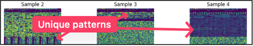
Fig 1. First N Bytes of Traditional Malware

While the first N bytes approach is effective at discerning traditional malware from benign files, it struggles significantly when faced with more sophisticated, obfuscated threats.

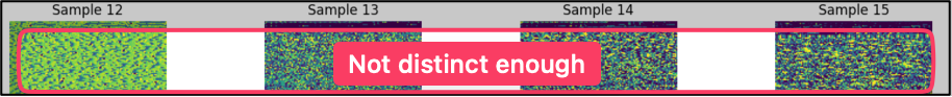
Fig 2. First N Bytes is Insufficient to Distinguish Obfuscated Malware

To overcome these challenges, a multi-segment feature extraction approach, guided by Shannon entropy [9], was implemented. This strategy enables more robust detection by capturing meaningful patterns throughout the entire file, rather than relying exclusively on its initial segment.

Our methodology consists of 2 major components:

• Entropy-based Sliding Window Feature Extraction, which finds and extracts multiple informative byte regions from each malware sample.
• A CNN Architecture that ingests the composite byte-region image and learns to classify the malware.

While we could split a file into fixed-size chunks, a sliding window guided by entropy highlights the most suspicious regions, enabling the extraction of fewer—yet more informative—byte segments. This approach both reduces noise and pinpoints high-risk code segments, ensuring the classifier focuses on content most likely to distinguish a specific malware.
Building on the concepts from a paper which analyzes an entire file’s entropy by creating a time series [10] and applying wavelet transforms to capture variations, our approach similarly capitalizes on distinct 'entropy signatures' in different malware families.

The idea is that different malware categories can have distinct entropy 'signatures' (some might have two spikes corresponding to two encrypted sections, others a single long spike).  We will extend those same concepts to our process, since those same 'signatures' should translate to our byte-image representation.

While the entropy time series in the paper was captured using non-overlapping, fixed-size chunks, our sliding window ensures we don’t miss critical high-entropy regions, even when we sample only part of the file.

Consider the following example entropy profile of a binary file: The high entropy regions (light blue region) stand out from low-entropy areas. A sliding window approach allows such regions to be captured regardless of alignment, unlike fixed-size segmentation (red blocks, in this case aligned to every 1000 blocks) which unable to accurately capture the full entropy 'signature' (yellow region).

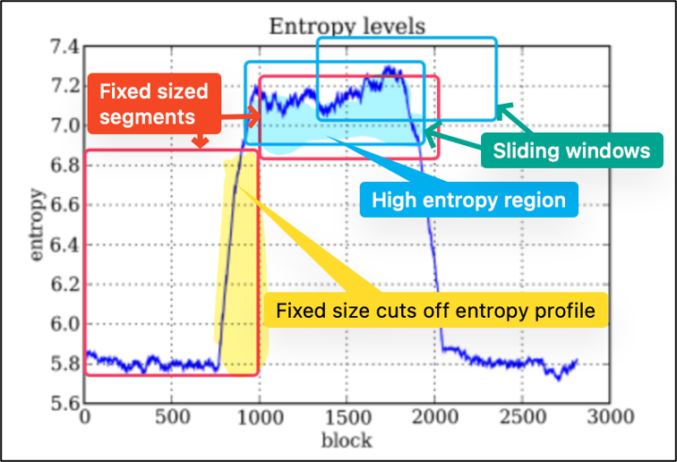
Fig 3. Example entropy profile of a binary file across its length (dark blue curve is entropy per block). *Image modified from [11]*

In the following section, we walk through each of our sliding window approach, from defining the window, to applying a dynamic threshold and assembling those regions into concise feature vectors:

Fig 4. Overview of Entropy-Based Sliding Window Feature Extraction Process.

1. Defining Sliding Windows

   
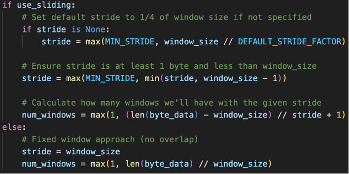
   Fig 5. Code to Define Sliding Window

   • 12,544 bytes sized windows are created that will 'slide' across the file.
   • Each stride will be 1/4 of the window size (3,136 bytes) so in a single window, 4 entropy 'snapshots' will be captured.
   • Sliding window will begin at byte 0 and extract from byte 0 till byte 12,543 in for the 1st region, moving the window forward 3,136 bytes each time, until the end of the file.

     
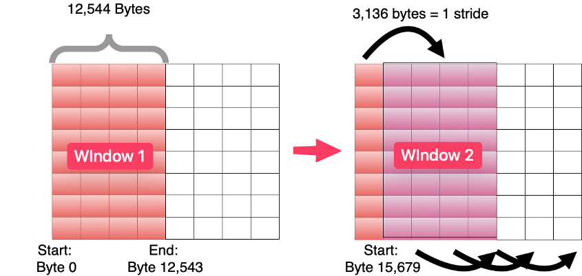
     Fig 6. Example of sliding window implementation

2. Entropy Calculation for Each Window
   • For each window, shannon entropy is calculated to calculate entropy value and stored along with the windows start/end position.

     
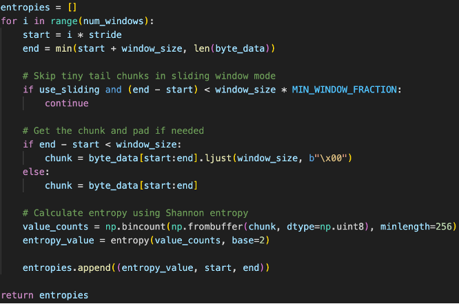
     Fig 7. Snippet of Entropy Calculation Code

3.  Entropy Threshold Calculation

   
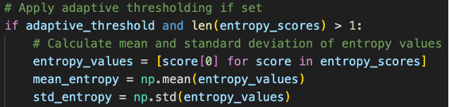
   Fig 8. Snippet of Entropy Threshold Code

   
    
   • Entropy scores from all window positions are collected.
   • Mean (average entropy for this specific file) and standard deviation (entropy variation within this specific file) is then calculated.
      
4. Setting a Dynamic Threshold

   
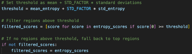
   Fig 9. Snippet of Dynamic Threshold Setting

   • Threshold is set at mean + 1.5 standard deviation for each file. This means files with overall higher entropy will have a higher threshold and lower entropy, lower threshold in order to select for the most anomalous parts relative to each file.
   • If no windows pass the threshold, we will just use the top entropy window (safety net to ensure that we always capture some features, even if file has relatively uniform entropy, which itself can be a characteristic that might distinguish certain malware categories i.e. absence of distinctive regions becomes a feature in itself such as files with artificially manipulated entropy to evade detection).
      
5. Rank and Select Representative Windows
   • Filtered windows are then sorted by entropy values
   • Highest entropy window is selected first, then for each subsequent window, calculate overlap with highest entropy window, if overlap >50%, discard this window to enforce more diversity.

     
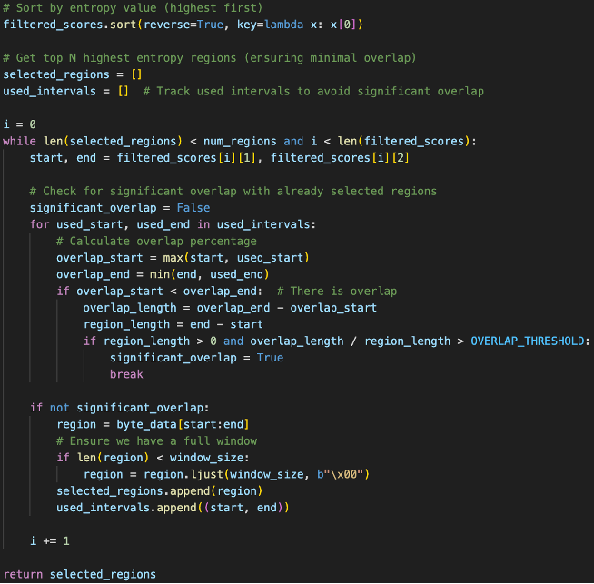
     Fig 10. Function Selecting Entropy Windows

6. Feature Vector Construction
   We now have 4 segments for each file:
   1. First 12KB Bytes: Capturing headers, imports, and static indicators.
   2. Highest Entropy 12KB Byte Region: The selection of the highest entropy region was identified based on packed malware samples, where obfuscation techniques such as packing and encryption often manifest as high-entropy regions.
   3. 2nd Highest Entropy 12KB Byte Region: Captures additional entropy 'signature'.
   4. Last 12KB Bytes: Captures potential artifacts and obfuscation techniques used by threat actors such as APT28.

      
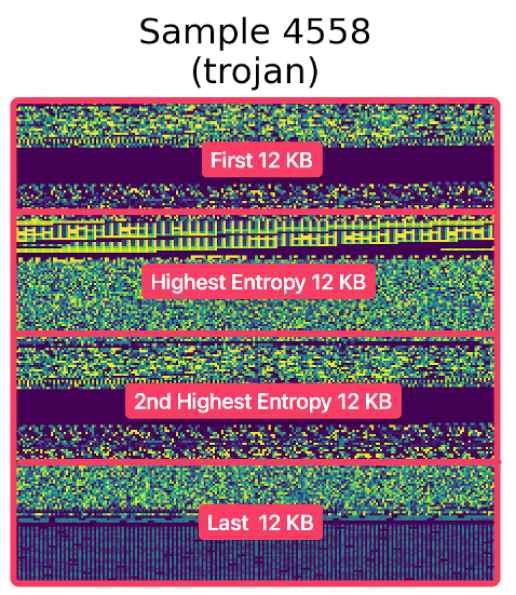
      Fig 11. Captured Segments of a Malware Sample

These segments are combined into a single 50,176-byte vector, where:

1. A list of feature_arrays is first initialized. We will use np.frombuffer() to convert the binary data in first_region into a NumPy array.
2. We then loop through the compiled high_entropy_regions and covert them into a NumPy array before adding them to the same feature_arrays.
3. The last region is also converted and appended the same way.
4. We will use np.hstack() to concatenate them along the first axis, creating a feature vector.
5. We will double check the size, truncating the vector if oversized, and padding with zeroes if undersized.

   
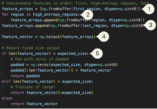
   Fig 12. Snippet for Final Feature Vector Construction

Given a malware file of 500 KB:

• The sliding window now generates ~160 entropy measurements instead of only 40 with fixed windows chunks.
• Adaptive threshold captures what is 'significant', for example if the entropy is 6 bits and only 1 window is 7.5 bits while the 2nd highest region is 5.9 bits, we do not capture the 2nd highest region since it is not meaningfully different from the rest of the file.

BODMAS Dataset

We used the BODMAS (Blue Hexagon Open Dataset for Malware Analysis) dataset [12] for this project. The BODMAS (Blue Hexagon Open Dataset for Malware Analysis) dataset is a comprehensive dataset of 57,293 malicious and 77,142 benign Windows PE files, including disarmed malware binaries, feature vectors and metadata, kindly provided by Zhi Chen and Dr Gang from the University of Illinois Urbana-Champaign for this exploration, the dataset offers more up-to-date and well-annotated samples compared to many existing sources, which often lack family/feature details, withhold binaries, or contain outdated threats.
 

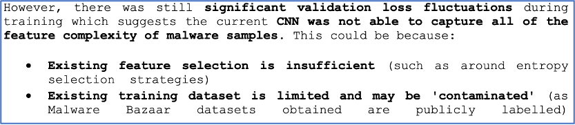
Fig 13. Excerpt from a Previous Attack Observation Highlighting Potential Issues with Public Labels

Data Preprocessing

While there are 14 malware categories within the BODMAS dataset, because not all malware categories contain sufficient samples, we only focus on selected categories and store them in a dictionary mapping:

• Worm
• Trojan
• Downloader
• Dropper
• Backdoor
• Ransomware
• Information Stealer
• Virus

 
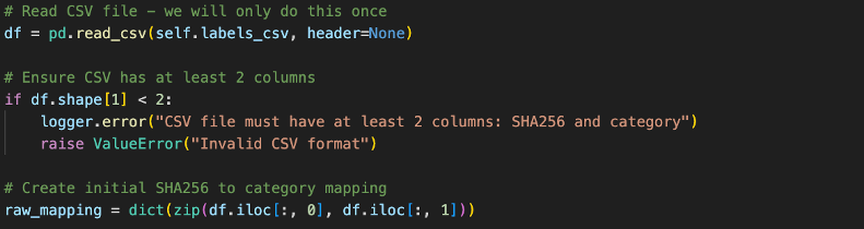
Fig 14. Data Preprocessing Code for Creating Category Mappings

We will categorize the benign files first since any files that are unlabeled are benign files, before categorizing the malicious files.

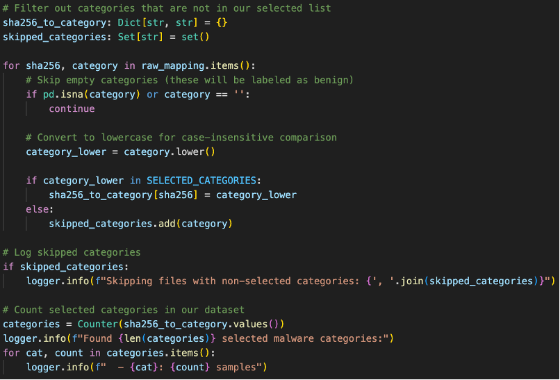
Fig 15. Data Preprocessing Code for Filtering Out Benign Files

We will then create integer labels for the all the categories in ascending order since we are using sparse_categorical_crossentropy. The 'benign' category is placed last, which assigns all the uncategorized files as benign.

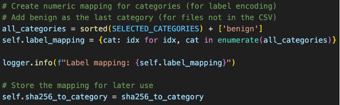
Fig 16. Integer Labeling for All Assigned Categories

Tangent: Importance of Logging

During first several runs of the training process, there appears to be excessive files showing up as low entropy from the logging added to catch edge cases. Duplicate '._<hash>' files of our malware samples were being picked up by our self.executables_dir.glob("*.exe") file glob pattern as treated as valid executables files since they had the same extension as our original malware samples.

Fig 17. Logging Messages Showing ._<hash> Files

These files were AppleDouble files [13] that are automatically created when macOS interacts with files on non-macOS filesystems, which was not accounted for during the switch to an external drive to better organize the large BODMAS malware dataset.

This negatively impacted the initial training process and would probably have gone unnoticed if not for the deliberate logging added during the training process as they were hidden even with system commands to show hidden files from the finder.

A fix was subsequently added to the data preparation script to filter out the files.

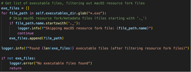
Fig 18. Fix to Filter out Resource Fork Files

To address class imbalance in our dataset, before CNN training, we used  sklearn.utils.class_weight to compute the class weights [14] based on the precomputed y_labels, where the weights scales inversely proportional to the class frequencies. The weights are calculated after train/test split to properly reflect training and testing distributions.

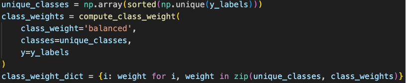
Fig 19. Class Weight Balancing Based on Class Frequencies

The combined data from previous data preparation steps were split into training and test sets. We have not shuffled the data before this stage to  maintain class distribution and will use stratified sampling [15] (stratify=y_labels) in order to maintain class distribution in our test splits. This ensures that our test set properly represents our entire population. We will use a random seed of 42 because *insert pop culture reference here*. [16]

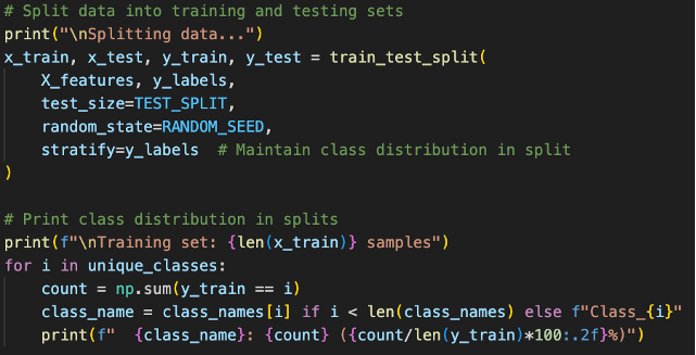
Fig 20. Stratified Sampling on Train Test Split

The final CNN model consists of multiple convolutional layers with batch normalization and dropout to enhance feature extraction and prevent overfitting. The architecture is as follows:

1. Convolutional Layers Progression: 32, 64, 128, 256 filters
2. Kernel Size: 3x3
3. Padding: 'same'
4. Activation Layer: 'relu'
5. Batch Normalization
6. MaxPooling: 2x2
7. Progressive Dropout Rates: 0.2, 0.3, 0.4, 0.5
8. Activation Layer: 'Softmax'
9. Loss: Sparse Categorical Cross Entropy
10. Optimizer: Adam
11. Learning Rate: 0.001

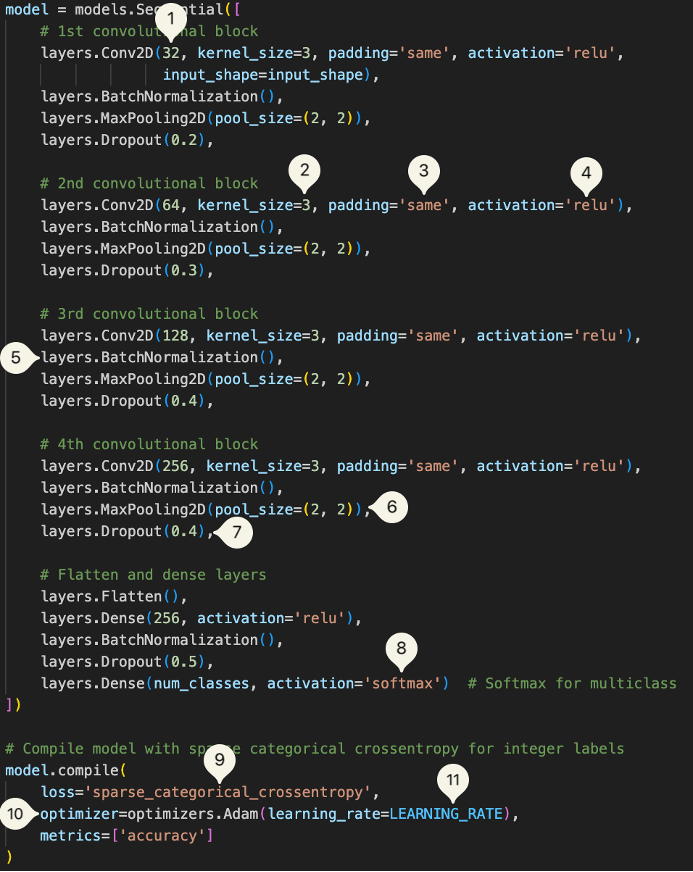
Fig 21. CNN Model Parameters

The model was compiled with an Adam optimizer (learning rate = 0.0001) and trained using the following hyperparameter optimization:

• BatchNormalization to stabilize learning.
• ReduceLROnPlateau: Adjusts the learning rate when validation loss plateaus after 3 epochs.

  
  Fig 22. ReduceLROnPlateau triggering on Epoch 9

• EarlyStopping: Prevents overfitting by stopping training if validation loss stops improving after 10 epochs (patience = 10, restores best weights).
• ModelCheckpoint: Saves the best-performing model based on validation loss.
   

Model Evaluation and Benchmarking

The model was evaluated on a held-out test set of 11,442 malware samples (20% of the BODMAS malware dataset, never seen during training)

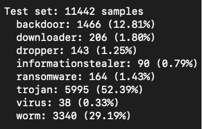
Fig 23. Distributions of Test Set

Key evaluation metrics include:

• Precision
• Recall
• Confusion matrix
• Additionally, we also tracked per-class accuracy, along with F1-score for each class

With a final test score of 90.88% and test loss of 0.3317, the results were very promising, demonstrating that the model not only achieves high overall accuracy, but does so consistently across all malware types. Below, we dive into each evaluation aspect and then compare our approach with other malware detection solutions.

The model faced the most difficulty when classifying  dropper and downloader, with both showing a high recall and low precision [17], indicating that the model misclassifies other samples as droppers and downloaders.

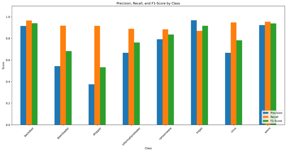
Fig 24. Per Class Metrics

The figure below plots the model's training progress over 30 epochs. The training accuracy (blue curve) shows a smooth upward trend, reaching 92.42% accuracy by the final epoch, while the validation accuracy (orange curve) climbs to 91.76%, tracking closely with the training curve, indicating to us that our model is generalizing well (not overfitting) and that there is likely still room to increase model capacity.

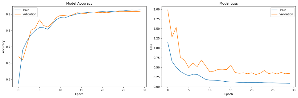
Fig 25. Model Training and Validation Performance History

Let us break down the per class accuracy:

• Given 1466 unseen backdoors tested: 96.6% (1416) were accurately determined
• Given 206 unseen downloaders tested: 91.7% (189) were accurately determined
• Given 143 unseen droppers tested: 91.6% (131) were accurately determined
• Given 90 information stealers tested: 88.9% (80) were accurately determined
• Given 164 unseen ransomware tested: 88.4% (145) were accurately determined
• Given 5995 unseen trojan tested: 87.0% (5215) were accurately determined
• Given 38 unseen virus tested: 94.7% (36) were accurately determined
• Given 3340 unseen worm tested: 95.4% (3187) were accurately determined

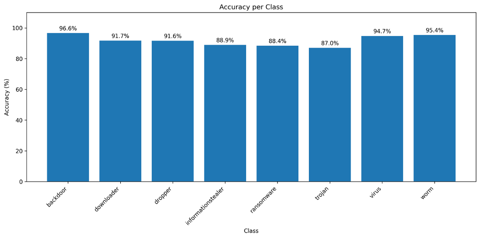
Fig 26. Model Training and Validation Performance History

While accuracy is a common and intuitive metric for evaluating machine learning models, it can be misleading, particularly in multi-class classification scenarios like ours.

Consider a different scenario: a multi-class model classifying data into eight distinct categories achieves an accuracy of 50%. Initially, this result might seem unimpressive and akin to random guessing. However, compared to random guessing—which would yield only 12.5% accuracy—a 50% accuracy indicates significant predictive capability.

Fig 27. "I Swear All These Look The Same"

Nevertheless, accuracy alone doesn't reveal the entire performance story. A confusion matrix provides valuable insights by clearly displaying how the model’s predictions are distributed among different categories. It helps identify specific categories frequently confused with each other, enabling targeted improvements such as the need for additional distinguishing features, or reconsideration of category definitions, possibly merging categories that are inherently similar.

Analyzing the confusion matrix [18], we observe clear diagonal dominance indicating accurate class separation overall, yet some notable misclassification patterns emerge:

1. Trojans are often misclassified as other classes:
   • This could be due to malware categories generally sharing similar byte-level patterns with Trojan (which deliberately disguises themselves as other software)
   • Our class-weighting strategies might also lead the model to overly emphasize minority-class characteristics (as the model is penalized heavily for misclassifying the minority), inadvertently causing proportionally more misclassifications into minority class like downloaders and droppers.
      
2. Worms are notably misclassified as Droppers, and Trojans:
   • Worms and Droppers, in particular, may possess common characteristics that are challenging to differentiate clearly, such as similar network call patterns or byte-level features.

     
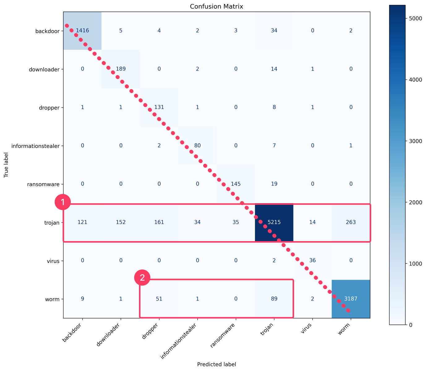
     Fig 28. Model's Confusion Matrix [18]

To place our model’s performance in context, we compared its results against DeepGray [19] due to its contemporary relevance and extensive performance evaluation using several established pre-trained image recognition models, such as:

•    VGG16 [20]
•    InceptionV3 [21]
•    EfficientnetV2B0 [22]
•    Vision Transformers(ViT-B32) [23]

It is important to recognize that due to the slight difference in category labels chosen, it is not a direct 'apples to apples' comparison. However, these comparisons still help validate our model’s efficacy relative to latest methodologies and offer valuable insight in general effectiveness of our methodology and highlights areas where further refinement could drive even stronger results.

Overall, our self-taught model did admirably well, even when compared to established pre-trained image recognition models.

Our accuracy of 91% puts it right in the middle of the pack, although due to our class imbalance, our macro averages—which treat each class equally—were significantly lower than our weighted averages, which adjust performance by class frequency. This disparity highlights the nuances of multi-class evaluation: while the model is highly effective in aggregate, certain minority classes (e.g. droppers, downloaders) drive down the macro metrics.
 

Model	Accuracy	Score	Precision	Recall	F1-Score
VGG16 (DeepGray)	0.82	Macro Weighted	0.83 0.83	0.80 0.82	0.80 0.82
InceptionV3 (DeepGray)	0.90	Macro Weighted	0.90 0.90	0.90 0.90	0.90 0.90
Our Model	0.91	Macro Weighted	0.73 0.93	0.92 0.91	0.80 0.91
EfficientnetV2B0 (DeepGray)	0.93	Macro Weighted	0.93 0.93	0.93 0.93	0.93 0.93
ViT-B32 Vision Transformer (DeepGray)	0.95	Macro Weighted	0.96 0.95	0.96 0.95	0.96 0.95

Table 1. Comparison of our model against models used in DeepGray

By leveraging entropy-driven feature selection and a specialized CNN architecture, we demonstrated a robust multi-class malware classification approach that effectively distinguish obfuscated threats. Through dynamic thresholding of high-entropy regions, we ensure the model focuses on byte-level segments most indicative of malicious behavior, delivering an approximate 91% accuracy on a held-out test set. Notably, the model maintains strong performance across varied malware families—including trojans, worms, and ransomware.

Beyond pure accuracy metrics, the model’s confusion matrix reveals targeted misclassification challenges. Categories like droppers and downloaders show overlapping features, emphasizing the need for continuous refinement of feature engineering to reduce false positives. Nonetheless, these results are encouraging, even when compared to leading pre-trained image recognition models on analogous malware detection tasks, validating the general effectiveness of our methodology.

From a practical standpoint, the work also highlights the importance of rigorous data preprocessing, class balancing, and proper logging. Identifying and filtering out spurious files (e.g., AppleDouble files) proved crucial to maintaining dataset integrity. Similarly, stratified sampling and class-weight adjustments helped ensure fairer representation of minority classes, mitigating skewed distribution and improving both model accuracy and reliability.

Also, scripts for performing the data preparation and classification are shared on GitHub [24].

[1] https://www.sans.edu/cyber-security-programs/bachelors-degree/
[2] https://en.wikipedia.org/wiki/Feature_selection
[3] https://en.wikipedia.org/wiki/Convolutional_neural_network
[4] https://developers.google.com/machine-learning/crash-course/classification/multiclass
[5] https://isc.sans.edu/diary/31050
[6] https://isc.sans.edu/diary/31194
[7] https://www.researchgate.net/publication/378288472_A_comprehensive_review_of_machine_learning's_role_in_enhancing_network_security_and_threat_detection
[8] https://www.sans.org/cyber-security-courses/applied-data-science-machine-learning/
[9] https://www.quantamagazine.org/how-claude-shannons-concept-of-entropy-quantifies-information-20220906/
[10] https://www.researchgate.net/publication/365110043_Classification_of_Malware_by_Using_Structural_Entropy_on_Convolutional_Neural_Networks
[11] https://deadhacker.com/2007/05/13/finding-entropy-in-binary-files/
[12] L. Yang, A. Ciptadi, I. Laziuk, A. Ahmadzadeh and G. Wang, "BODMAS: An Open Dataset for Learning based Temporal Analysis of PE Malware," 2021 IEEE Security and Privacy Workshops (SPW), San Francisco, CA, USA, 2021, pp. 78-84, doi: 10.1109/SPW53761.2021.00
[13] https://en.wikipedia.org/wiki/AppleSingle_and_AppleDouble_formats
[14] https://www.tensorflow.org/tutorials/structured_data/imbalanced_data
[15] https://scikit-learn.org/stable/modules/generated/sklearn.model_selection.train_test_split.html
[16] https://en.wikipedia.org/wiki/Phrases_from_The_Hitchhiker%27s_Guide_to_the_Galaxy#Answer_to_the_Ultimate_Question_of_Life,_the_Universe,_and_Everything_(42)
[17] https://en.wikipedia.org/wiki/Precision_and_recall
[18] https://en.wikipedia.org/wiki/Confusion_matrix
[19] https://www.researchgate.net/publication/380818154_DeepGray_Malware_Classification_Using_Grayscale_Images_with_Deep_Learning
[20] https://arxiv.org/pdf/1409.1556
[21] https://arxiv.org/pdf/1512.00567
[22] https://arxiv.org/pdf/2104.00298
[23] https://arxiv.org/pdf/2101.03771
[24] https://github.com/weekijoon/entropy-malware-classifier-cnn

--
Jesse La Grew
Handler